Software > Latent Semantic Analysis
Description | Pros and Cons | Applications | Details | Usage Hints | References | Acknowledgments| Description |
Latent Semantic Analysis (LSA) can be applied to induce and represent aspects of the meaning of words (Berry et al., 1995; Deerwester et al., 1990; Landauer & Dumais, 1997; Landauer et al.,1998). LSA is a variant of the vector space model that converts a representative sample of documents to a term-by-document matrix in which each cell indicates the frequency with which each term (rows) occurs in each document (columns). Thus a document becomes a column vector and can be compared with a user's query represented as a vector of the same dimension.
In the case of digital libraries, terms may stand for words in abstracts or titles, author names, or cited references. Only author names, titles, abstracts, and cited references occurring in more than one document are included in the analysis.
LSA extends the vector space model by modeling term-document relationships using a reduced approximation for the column and row space computed by the singular value decomposition of the term by document matrix. This is explained in detail subsequently.
Singular Value Decomposition (SVD) is a form of factor analysis, or more properly, the mathematical generalization of which factor analysis is a special case (Berry et al., 1995). It constructs an n dimensional abstract semantic space in which each original term and each original (and any new) document are presented as vectors.
In SVD a rectangular term-by-document matrix X is decomposed into the product of three other matrices W, S, and P' with {X} = {W} {S} {P}' (see figure below).
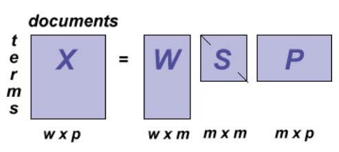
W is a orthonormal matrix and its rows correspond to the rows of X, but it has m columns corresponding to new, specially derived variables such that there is no correlation between any two columns; i.e., each is linearly independent of the others. P is an orthonormal matrix and has columns corresponding to the original columns but m rows composed of derived singular vectors. The third matrix S is an m by m diagonal matrix with non-zero entries (called singular values) only along one central diagonal. A large singular value indicates a large effect of this dimension on the sum squared error of the approximation. The role of these singular values is to relate the scale of the factors in the other two matrices to each other such that when the three components are matrix multiplied, the original matrix is reconstructed.
Following the decomposition by SVD, the n most important dimensions (those with the highest singular values in S) are selected. All other factors are omitted, i.e., the other singular values in the diagonal matrix along with the corresponding singular vectors of the other two matrices are deleted. The amount of dimensionality reduction, i.e. the choice of n is critical and an open issue in the factor analytic literature. Ideally, n should be large enough to fit the real structure in the data, but small enough such that noise, sampling errors or unimportant details are not modeled (Deerwester et al., 1990). Use good retrieval and browsing performance as an operational criterion.
The reduced dimensionality solution then generates a vector of n real values to represent each document. The reduced matrix ideally represents the important and reliable patterns underlying the data in X. It corresponds to a least-squares best approximation to the original matrix X.
Similarity matrix: The similarity between documents can be computed on the basis of the three matrices as follows:
- Matrix multiply W (its rows correspond to the terms (rows) of X) by the reduced matrix S.
- Normalize resulting vectors, i.e., divide each vector by its length. This way all vectors are mapped onto a hypersphere.
- Determine the document-document matrix of inner products that defines the similarities between all documents.
The dot product between two row vectors of the reduced matrix reflects the degree to which two documents have a similar pattern of terms. The matrix XX' is the square symmetric matrix containing all these document-document dot products. Since S is diagonal and W is orthonormal, the following holds: XX'=WS2W'. Thus the i, j cell of XX' can be obtained by taking the dot product between the i and j rows of the matrix WS. That is, if one considers the rows of WS as coordinates for documents, dot products between these points give the comparison between documents.
Data Visualization: Different algorithms can be applied to display the resulting semantic networks. Among them are Spring Embedding Algorithm and Pathfinder Network Scaling. Sometimes you may wish to display a certain partition of data into clusters/categories. Use Matlab to cluster your data hierarchically and select the best partition of the hierarchy according to the utility measure given below.
Hierarchical Clustering: Apply nearest-neighbor-based, agglomerative, hierarchical, unsupervised conceptual clustering to create a hierarchy of clusters grouping documents of similar semantic structure. Clustering starts with a set of singleton clusters, each containing a single document di D, i=1, ..., N, where D equals the entire set of documents and N equals the number of all documents. The two most similar clusters over the entire set D are merged to form a new cluster that covers both. This process is repeated for each of the remaining N-1 documents. A complete linkage algorithm is applied to determine the overall similarity of document clusters based on the document similarity matrix.
Merging of document clusters continues until a single, all-inclusive cluster remains. At termination, a uniform, binary hierarchy of document clusters is produced.
The figure below shows an example of how five documents may be clustered hierarchically. The cluster hierarchy is shown on the left hand side. Corresponding partitions are given on the right hand side. Note that each documents to itself has a similarity of one.
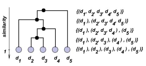
Hierarchical Clustering
Selection of the Best Partition:The partition showing the highest within cluster similarity and lowest between-cluster similarity is determined by means of a utility measure that contrasts the sum of within-cluster similarities wSim by the sum of between-cluster similarities bSim: utility = wSim / (wSim + bSim). The partition that shows the highest utility is selected for data visualization.
| Pros & Cons |
The advantage of SVD lies in the fact that documents are not represented by individual terms but by a smaller number of independent "artificial values" that can be specified by any one of several terms or combinations thereof. In this way, relevant documents that do not contain the terms of the query are retrieved via other terms in the query that can be properly identified. The resulting retrieval scheme allows one to order documents continuously by similarity to a query. A similarity threshold or a number of solutions can be specified depending on the user and task.
In such a way, SVD overcomes two fundamental problems faced by traditional lexical matching indexing schemes: synonymy (variability of word choice - that is different words can be used to express a concept and query terms may not match document descriptions) and polysemy (words can have multiple meanings and a user's query may match irrelevant meanings and thus retrieve irrelevant documents) (Deerwester et al., 1990).
| Applications |
- LVis Digital Library Visualizer (Börner et al., 2000)
| Details |
The SVDPACK by M. Berry (1993) berry@cs.utk.edu comprises four numerical (iterative) methods for computing the singular value decomposition of large sparse matrices using double precision (Well, this was true some years ago ... it is much faster now!)
The package allows one to decompose matrices on the order of 50,000 by 50,000 (e.g. 50,000 words and 50,000 contexts) into representations in 300 dimensions with about two to four hours of computation on a high-end Unix work-station with around 100 Megabytes of RAM.
The computational complexity is O(3Dz), where z is the number of non-zero elements in the word (W) X context (C) matrix and D is the number of dimensions returned. The maximum matrix size one can compute is usually limited by the memory (RAM) requirement, which for the fastest of the methods in the Berry package is (10+D+q)N + (4+q)q, where N=W+C and q=min (N, 600), plus space for the W X C matrix.
Other packages:
MatLab restricted to small matrices.
| Usage Hints |
From the SVDPACK, the sparse SVD via single-vector Lanczos algorithm will be used because of its comparatively low memory and processing requirements and low to moderate accuracies. The document by term input matrix has to be represented in a compressed Harwell-Boeing storage fomat (Berry et al, 1993) Appendix B.
The package and all java files can be found on ella in '/home/www/ella/htdocs/classes/L697/code/lsa'.
There are four separate steps involved in determining and visualizing the semantic relationships between documents:
1. Generate compressed Harwell-Boeing storage format:
- Use 'DocumentParser.java', 'DocumentNW.java', 'Document, java' and 'MatrixSort.java' by Katy Börner to read in representative samples of documents like slis-courses.dat, to determine its document-term frequency matrix (cell entries are term frequencies in the documents), and to write the result out in compressed Harwell-Boeing storage format, like 'slis-courses.hbf'.
- Just copy the four files and input *.dat files, compile with 'javac DocumentParser.java' and run with 'java DocumentParser'. Change input/output file names in 'DocumentParser.java' if needed.
- Copy all files in ../lsa/svdpack into your svdpack directory.
------ ------------ ---------
las2.c lap2, matrix lao2,lav2,lav2-data
- Compiling with 'gcc las2.c timersun.o -lm' creates a.out.
- The program expects a file named 'matrix' in Harwell-Boeing storage format. Just rename 'slis-courses.hbf' into 'matrix'.
- Run with 'a.out'. The result (right-singular vectors, left-singular vectors, and singular values) is stored in 'lav2-data'. (If the current path is not set in your shell script properly, start c-programs with './a.out'.)
- You can influence how many singular values are generated by manipulating the second number in the parameter file lap2. The file contains a single line.
where <name> is the name of the data set;
lanmax is an integer specifying maximum number of lanczos
step allowed;
maxprs indicates maximum number of singular triplets of A
(eigenpairs of the equivalent matrix B) desired;
endl,endr are two end-points of an interval within which all
unwanted eigenvalues of the particular matrix B lie;
vectors contains the string TRUE or FALSE to indicate when
singular triplets are needed (TRUE) and when only
singular values are needed (FALSE);
kappa contains the relative accuracy of ritz values
acceptable as eigenvalues of the matrix B.
- Copy the right-singular vectors and singular values into a '*.lsa' file that has the following format:
RSV 2 7
-0.027681 0.020486 -0.056959 0.012744 -0.084846 -0.035440 -0.015950
0.108894 0.146756 0.169545 0.114511 0.167698 0.126818 0.193714
SV 2
6.524949
7.260814
- Typically, you will have many more dimensions but never more than in your input matrix :)
- Use 'SimParser.java' and 'SimParserMain.java' by Katy Börner to read in the Right Singular Vectors as well as the Singular Values (slis-courses.lsa) as computed by LSA, to matrix multiply W by the reduced matrix S, to normalize resulting vectors & to determine the document-document matrix of inner products that defines the similarities between all documents. Just copy the two files and sample input *.dat file, compile with 'javac SimParserMain.java' and run with 'java SimParserMain > out.txt'. Change input file name in 'SimParserMain.java' if needed. The resulting inner product matrix corresponds to the matrix in 'out.txt' after the line 'Inner Product:' For the slis-courses it looks like slis-courses.sim. Note that all diagonal values are 1.
- Note that 'SimParser.java' contains a hierarchical clustering method based on the Inner Product matrix (complete Linkage method) that can be used to quickly compute a cluster hierarchy.
4. Display the semantic document relationships using Spring Embedding Algorithm or Pathfinder Network Scaling. A similarity matrix such as slis-courses.sim and the corresponding data file slis-courses.dat can be merged and converted into the corresponding xml file using SimConverter.java in '/home/www/ella/htdocs/classes/L697/code/toolkit/demo/'. Simply compile and run SimConverter and enter the Matrix File '*.sim' file and Source Data File '*.dat' second. The result is named list.xml.
| References |
- Berry, M. et al. SVDPACKC (Version 1.0) User's Guide, University of Tennessee Tech. Report CS-93-194, 1993 (Revised October 1996). See also http://www.netlib.org/svdpack/index.html.
- Berry, M., Dumais, S.T., & O'Brien, G.W. (1995). Using linear algebra for intelligent information retrieval. SIAM: Review, 37(4), 573-595. See also http://www.cs.utk.edu/~berry/
- Börner, K., Dillon, A. & Dolinsky, M. (2000) LVis - Digital Library Visualizer. Information Visualisation 2000, Symposium on Digital Libraries, London, England, 19 -21 July, pp. 77-81. (http://ella.slis.indiana.edu/~katy/IV-LVis/)
- Deerwester, S., Dumais, S. T., Furnas, G. W., Landauer, T. K., & Harshman, R. (1990). Indexing By Latent Semantic Analysis. Journal of the American Society For Information Science, 41, 391-407. See also http://lsa.colorado.edu/
- Landauer, T.K., & Dumais, S.T. (1997). A solution to Plato's problem: The latent semantic analysis theory of the acquisition, induction, and representation of knowledge. Psychological Review, 104, 211-240. See also http://lsa.colorado.edu/
- Landauer, T. K., Foltz, P. W., & Laham, D. (1998). Introduction to Latent Semantic Analysis. Discourse Processes, 25, 259-284. See also http://lsa.colorado.edu/
- Landauer, T. K., Laham, D. & Foltz, P. W. (1998). Learning human-like knowledge by Singular Value Decomposition: A progress report. In M. I. Jordan, M. J. Kearns & S. A. Solla (Eds.), Advances in Neural Information Processing Systems 10, pp. 45-51. Cambridge: MIT Press. See also http://lsa.colorado.edu/
- Rehder, B., Schreiner, M. E., Wolfe, M. B., Laham, D., Landauer, T. K., & Kintsch, W. (1998). Using Latent Semantic Analysis to assess knowledge: Some technical considerations. Discourse Processes, 25, 337-354. See also http://lsa.colorado.edu/
- Kintsch, W. (in press). Predication. Cognitive Science. See also http://lsa.colorado.edu/
- Kintsch, W. (in press). Metaphor comprehension: A computational theory. Psyhonomic Bulletin and Review. See also http://lsa.colorado.edu/
| Acknowledgments |
The original LSA code (SVDPACK) was provided by Michael Berry berry@cs.utk.edu. Katy Börner implemented the parsers as well as code to compute the document by document or term-by-term matrices. Sriram Raghuraman integrated the code into the XML toolkit.
![]()
Information
Visualization Cyberinfrastructure @ SLIS,
Indiana University
Last Modified January
14, 2004