Software > Network Analysis Toolkit
Description | Pros and Cons | Applications | Details | Usage Hints | References | AcknowledgmentsDescription |
The Network Analysis Toolkit (henceforth, 'toolkit') is a toolkit that allows one to analyze networks of various types. It allows one to quickly examine basic properties of any network such as the number of nodes, edges and loops and also perform more extensive analyses such as computing the diameter of the network or various types of clustering coefficients. These networks may be generated using modelling tools or loaded from files of various formats.
Pros & Cons |
- Many commonly used values can be computed using the toolkit, however a large number of parameters are not computed.
- There is no real limit on the size of the network, (it is limited solely by the amount of available memory on the computer on which it is being run). However, for extremely large networks, the computation can take a very long time. For very large networks, one is better off writing programs in a faster language with a smaller memory footprint such as C or even Perl.
Applications |
Analysis of static networks of arbitrary size.
Details |
The toolkit uses the JUNG (Java Universal Network/Graph Framework) API in the backend. Each of the network measures has its own algorithm and/or formula and hence the best way to understand how these measures are computed is to go through the well-documented source code and read the references given below. A brief description of currently implemented network measures is given below. A very good place to look up definitions for terminology in graph theory is University of Tennessee Mathematics Department's Graph Theory Glossary. Also see (Pastor-Satorras & Vespignani, 2004)
| Directed | A graph is said to be directed when all of its edges are directed i.e. each edge has a source and a destination and the edge points from the source to the destination. This means that the relationship between the two nodes in the graph is uni-directional. |
| Connected | A graph in which there is a path from every node to every other node in the graph. A graph which does not satisfy this condition is said to be disconnected. |
| Self-Loop | A self loop is an edge whose source and destination are the same node. Hence a loop connects a node to itself. |
| Parallel Edge | Two edges which have the same source and destination nodes are said to be parallel. |
| Degree | The degree of a node is the number of edges connected to it. The in-degree of a node is the number of incoming edges and the out-degree is the number of outgoing edges. In and out degrees apply only to a directed graph. |
| Average Degree | The average of the degree of all nodes in the graph. |
| Diameter | The "longest shortest path" or the largest number of edges that must be traversed to get from any node to any other node in a graph using the shortest path not considering loops, backtracks and detours. |
| Characteristic Path Length | The average of all path lengths in the graph. It is obvious from this definition that computing this value can take a long time since it involves looking at every possible path from every node to every other node in the graph. |
| Scale Free Exponent | The exponent in the power law equation used to fit the distribution of degree of nodes in a graph. |
| Clustering Coefficient | The ratio of the actual number of edges existing between neighbours of a node to the number of all possible edges between those neighbours, averaged over all the nodes in a graph. This coefficient measures how "cliquish" the graph is, as in how closely the neighbours of a particular node interact with each other, see (Watts & Strogatz, 1998). |
| Mutual Connection Coefficient | Describes the intersection between the "downstream" and "upstream" neighbours of a node. A "downstream" neighbour is one to which there is a directed edge from the current node. An upstream neighbour is one from which there is a directed edge to the current node. This coefficient basically measures how bi-directional the interaction between a node and its neighbours is, averaged over all the nodes in the graph, see (Zhou, 2002). |
| Incoming Clustering Coefficient | The degree of cliquishness of the upstream neighbours of a given node. This coefficient measures the level of interaction between upstream neighbours of a node averaged over all the nodes in the graph, see (Zhou, 2002). |
| Outgoing Clustering Coefficient | The degree of cliquishness of the downstream neighbours of a given node. This coefficient measures the level of interaction between the downstream neighbours of a node averaged over all the nodes in the graph, see (Zhou, 2002). |
Usage Hints |
The toolkit can be found in the IVC under the 'Toolkits'
menu item. The toolkit is enabled only if a network data model is selected.
Networks can be either loaded from a file or similated via data modeling.
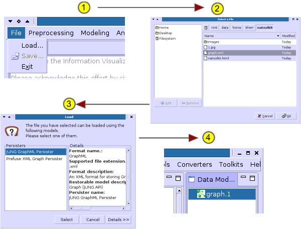
Load from a file.
- Click File->Load.
- Select the file to load.
- Select the type of data structure to load into using the appropriate persister.
- The model appears in the right side panel.
If you compose your own .net or .xml files, please make sure the file extension name is correct (.net or .xml) so that the IVC software can recognize the format. Note also that while you can use identical labels for different vertices in Pajek, it is not acceptable for the IVC.
In order to learn more about acceptable file formats, simply save a data model:
- File > Save to file
- Select JUNG GraphML Persister to save as *.xml file or JUNG Graph Pajek Format Persister to save as *.net file that can be read by Pajek.
- Select a directory and enter a file name and select Save.
Check out the representation of a fully connected three node network in *.net and *.xml format. Loading and saving a file can also be used to convert file formats.
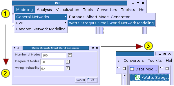
Use the IVC Modeling Plugins.
- Select a network modeling algorithm from the Modeling menu.
- Type in appropriate parameters and generate a graph.
- The model appears in the right-side pane.
Once your network has been loaded into the IVC, click on Toolkits->Network Analysis Toolkit to bring up the Network Analysis Toolkit. The toolkit has many sub-windows that allow you to compute and see different information on a given graph.
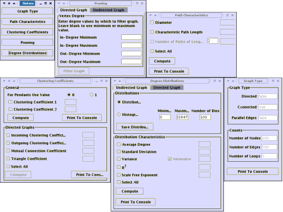
Be aware that certain measures such as diameter can take a long time to compute. Typically networks with a few thousand edges will take time to analyze. The toolkit runs the computations in a separate thread. Hence you should be able to simply minimize the window and work on something else concurrently. Since the computation can be processor-intensive, you will in most cases experience a slower response from other programs you are working on. If at any time, you run out of patience and wish to exit, close the window.
Once a computation has finished on any of the sub-windows click 'Print to Console' to print the results of your analysis to the IVC console. You can then copy paste those results to any file and save it for future use.
References |
- Duncan J. Watts, Steven H. Strogatz (1998) Collective dynamics of 'small-world' networks, Nature (393), 440 - 442.
- Romualdo Pastor-Satorras, Alessandro Vespignani (2004) Evolution and Structure of the Internet: A Statistical Physics Approach, Cambridge University Press. The appendix of this book has a general overview of graph theory and a good list of graph properties that are commonly used to describe graphs.
- Haijun Zhou (2002) Scaling exponents and clustering coefficients of a growing random network, Phys Rev E (66).
Acknowledgments |
This toolkit started out as an online system as part of a class project for the L597 class at IUB. Thanks to Katy Börner for her support throughout this project, Steve Borgatti of UCINet and Mark Newman for clarifying formulae for calculating clustering coefficient measures. Weimao Ke contributed helful hints to this page.
![]()
Information Visualization
Cyberinfrastructure @ SLIS,
Indiana University
Last Modified Sept 9th, 2005